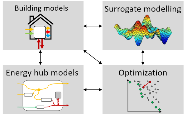

The buildings sector is one of the largest contributors to carbon emissions, up to 33% of global CO$_2$ emissions. Improved computational methods are needed to help design more energy-efficient buildings. besos is a Python library and associated web-based platform to help researchers and practitioners to explore energy use in buildings more effectively. This is achieved by providing an easy way of integrating many disparate aspects of building modelling, district modelling, optimization and machine learning into one common library.
The BESOS Platform is a Jupyter Hub that is able to run the besos code base, and has all the dependencies installed. The platform is freely accesible for academics in the building energy modelling space. To get started with BESOS the Platform we have provided this 2-page pamphlet that will get you from signup to your first notebook.
The besos library connects modelling and optimisation tools to allow for parameterizing running and optimizing models, sampling from their design spaces, and generating data for use in machine learning models. This supports designing building and district energy modelling experiments.
Python notebooks are great for mixing executable code, visual outputs and formatted explanations.
Run notebooks on our cloud resources, with a pre-configured environment where all libraries and other software (EnergyPlus, CPlex) are automatically kept up to date.
Explore your model by interactive visualization using sliders/buttons/dropdowns and pretty graphics. All the code is hidden but accessible to power users.
Start from templates, both ours and user-generated, which are editable in one click. Takes the pain out of complex workflows, integrating different models and adding app-like front-ends to your research.
Tutorials straight in the notebooks, from beginner to advanced, plus classroom-focused content.
More control for expert users, with terminal access to customize your environment like you would your local machine.
Our BESOS library for optimization and surrogate modelling of buildings provides wrappers for EnergyPlus via EPPy for energy simulation, Platypus for optimization and scikit-learn and TensorFlow for surrogate modelling.
Our PyEHub library for energy hub modelling of energy systems provides an easy way to define energy balancng and system sizing problems.
Easily move your work locally if desired, just download your notebooks and follow the instructions to replicate the environment.
Share folders with other users. Work together in real-time using Jupyter Lab. Coming soon
An executable paper! Make your notebook public with a static link and frozen dependencies. Include the link in your publications to encourage others to build on (and cite!) your work. Coming soon
Integrated HPC cluster submission for Compute Canada. Coming soon
The BESOS Platform is a cloud-based portal of modular, reusable software components for researchers to perform integrated building and energy systems analysis. Buildings, renewable energy generation and storage technologies and associated energy systems all pose complex, interacting design and operational challenges. Finding high-performing solutions to these problems requires a new generation of computational tools, blending aspects of simulation, optimization, machine learning and visualization. The project is funded by a grant from CANARIE.
Integration of the following core modules:
Modules are accessible by:
The main technologies that underpin the platform are:
These are examples of the many notebooks that are available on the BESOS platform.
They open on MyBinder, where you can edit and run them but not save them.
MyBinder might take a while to load, please be patient.
The BESOS platform is developed by the Energy in Cities group at the University of Victoria in beautiful British Columbia, Canada.
The group is led by Dr. Ralph Evins.
We are working with the following research teams to develop specific components and case studies:
To get started with BESOS the Platform we have provided this 2-page pamphlet that will get you from signup to your first notebook.
For all information on making use of besos library and locally installing it on your computer review the Read The Docs
Finding more info on EnergyHub modelling review the Read the Docs PyEhub to get details of specific classes.